|
|
How
depth information is obtained using stereo vision
Go to 3D Cameras
Making it work with the
stereo-matching technique and texture projection
|  General
stereo vision configuration General
stereo vision configuration
Depth perception from stereo vision is based on the triangulation
principle. Two cameras with projective optics as in, for example,
the camera/projector integrated unit, Ensenso
N10, are used and arranged side-by-side so that their view fields
overlap at the desired object distance. By taking a picture with
each camera the scene is captured from two different viewpoints.
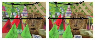
(Figure 1, right, illusrates an
example from the Middlebury Stereo Dataset "cones" where
a scene with paper cones is imaged with a stereo camera. The projection
rays of two cone tips into both camera images are drawn as an example).
For each surface point visible in both images, there is a ray
in 3D space connecting the surface point with each camera’s
centre of projection. In order to obtain the 3D position of the whole
captured scene two tasks need to be accomplished. Firstly, we need
to identify where each surface point that is visible in the left
image is located in the right image. Secondly, the exact camera
geometry must be known to compute the ray intersection point for
associated pixels of the left and right camera. Assuming that the
cameras are firmly attached to each other, the geometry is only
computed once during the calibration process.
Application-specific processing
A three-step process, described below, needs
to be carried out on the stereo image pair in order to obtain the
full 3D point cloud of the scene. The point
cloud then needs to be processed further to realize a specific application.
It can be used to match the surface of the scene against a known
object, either learned from a previous point cloud or a CAD model.
If the part can be located uniquely in the captured scene surface,
the complete position and rotation of the object can be computed
and it could, for example, be picked up by a robot.
Calibration
The geometry of the two-camera system is computed, deductively,
in the stereo calibration process. Firstly, a calibration object
is required and this is usually a planar calibration plate with
a checkerboard or dot pattern of known size. Secondly, synchronous
image pairs are captured from both cameras showing the pattern in different positions,
orientations and distances. Consequently, the pixel
locations of the "points" pattern dots in each image pair and their known
positions on the calibration plate can be used to compute both the
3D poses of all observed patterns and an accurate model of the stereo
camera. The model consists of the so-called intrinsic parameters
of each camera (the camera’s focal length and distortion)
and the extrinsic parameters (the rotation and shift in three dimensions
between the left and right camera). This calibration data is used
to triangulate corresponding points that have been identified in
both images and recover their metric 3D co-ordinates with respect
to the camera. |
|
|
|
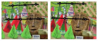
| Figure 2: Search space to match image
locations is only one dimensional. Left: The epipolar lines
are curved in the distorted raw images. Middle: Removing image
distortions results in straight epipolar lines. Right: Rectification
makes epipolar lines aligned with the image axes. Correspondence search
can be carried out along image scanlines. |
Processing
steps for depth computation
Three steps are now necessary for computing
3D location for each pixel of an image pair. These steps must be
performed in real time for each captured stereo image to obtain
a 3D point cloud or surface of the scene. |
| 1 |
Rectification |
| |
 In
order to triangulate the imaged points we need to identify corresponding
image parts in the left and right image. Considering a small image
patch from the left image, the entire right image could be searched for a sufficiently good match but this can be computationally intensive and too time
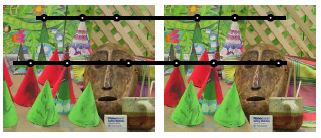
consuming to be done in real time. Consider the stereo image pair
example in Figure 3, (right), with the cone tip
visible in the top of the left image in the pair. Where do we have
to search for the cone tip in the second image of the pair? Intuitively
it does not seem necessary to search for the tip of the cone in
the bottom half of the right image when the cameras are mounted
side by side. In fact, the geometry of the two projective cameras
allows us to restrict the search to a one dimensional line in the
right image, the so called epipolar line. In
order to triangulate the imaged points we need to identify corresponding
image parts in the left and right image. Considering a small image
patch from the left image, the entire right image could be searched for a sufficiently good match but this can be computationally intensive and too time
consuming to be done in real time. Consider the stereo image pair
example in Figure 3, (right), with the cone tip
visible in the top of the left image in the pair. Where do we have
to search for the cone tip in the second image of the pair? Intuitively
it does not seem necessary to search for the tip of the cone in
the bottom half of the right image when the cameras are mounted
side by side. In fact, the geometry of the two projective cameras
allows us to restrict the search to a one dimensional line in the
right image, the so called epipolar line.
Figure 2 (above left) shows a few hand-marked point correspondences
and their epipolar lines. In the raw camera images the epipolar
lines will be curved due to distortions caused by the camera optics.
Searching correspondences along these curved lines will be quite
slow and complicated, but the the image distortions can be removed
by applying the inverse of the distortion learnt during the calibration
process. The resulting undistorted images have straight epipolar
lines, depicted in Figure 2 (above middle).
Although straight, the epipolar lines will have different
orientations in different parts of each image. This is caused by
the image planes (i.e. the camera sensors) neither being perfectly
co-planar nor identically oriented. To further accelerate the correspondence
search we can use the camera geometry from the calibration and apply
an additional perspective transformation to the images such that
the epipolar lines are aligned with the image scan lines*. This
step is called rectification.
The search for the tip of the white cone can now be carried out
by simply looking at the same scan line in the right image and finding
the best matching position. All further processing will take place
in the rectified images only, the resulting images are shown in
Figure 2 (above right).
*Mathematically speaking, the rays captured by the same scan
line of the rectified left and right image are all contained within
a single plane.
|
| 2 |
Stereo matching |
| |
For each pixel in
the left image, we can now search for the pixel on the same scan line
in the right image which captured the same object point.
Because a single pixel value is typically not discriminative enough
to reliably find the corresponding pixel, it is more beneficial to
match small windows (e.g. 7x7 pixels) around each pixel against all
possible windows in the right image on the same row. The entire row
need not be searched; only a limited number of pixels to the left
of the left image pixel’s x-coordinate, corresponding to the
slightly cross-eyes gaze necessary to focus near objects. This accelerates
the matching and restricts the depth range where points can be triangulated.
If a sufficiently good and unique match is found, the left image
pixel is associated with the corresponding right image pixel. The
association is stored in the disparity map in the form of an offset
between the pixels x-positions (Figure 4 below).
|
|
|
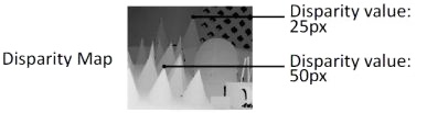
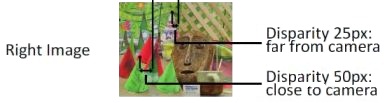
| Figure 4: Result
of image matching. The disparity map represents depth information
in form of pixel shifts between left and right image. A special
value (black) is used to indicate that a pixel could not be
identified in the right image. This will happen for occluded
areas or reflections on the object, which appears differently
in both cameras. |
This matching technique is called local stereo matching as
it only uses local information around each pixel. It works when a region in the
left and right images can be matched because it is sufficiently distinct
from other image parts on the same scan line. Local stereo matching
will fail on objects and in regions with a poor or a repetitive texture impedes it from finding a unique match.
Other methods, known as global stereo matching, can also
exploit neighboring information where the process doesn't just consider
each pixel (or image patch) individually to search for a matching
partner,but rather will try to find an assignment for all left and
right image pixels at once. This global assigment also takes into
account that surfaces are mostly smooth and thus neighbouring pixels
will often have similar depths. Global methods are more complex and
need more processing power than the local approach, but they require
less texture on the surfaces and deliver more accurate results, especially
at object boundaries. |
| |
|
| 3 |
Reprojection |
| |
 Regardless
of what matching technique is used, the result is always an association
between pixels of the left and right image, stored in the disparity
map. The values in the disparity map encode the offset in pixels,
where the corresponding location was found in the right image. Figure
4 (above) illustrates the disparity notion. The camera geometry
obtained during calibration can then be reused to convert the pixel-based
disparity values into actual metric X, Y and Z co-ordinates for every
pixel. This conversion is called reprojection. Regardless
of what matching technique is used, the result is always an association
between pixels of the left and right image, stored in the disparity
map. The values in the disparity map encode the offset in pixels,
where the corresponding location was found in the right image. Figure
4 (above) illustrates the disparity notion. The camera geometry
obtained during calibration can then be reused to convert the pixel-based
disparity values into actual metric X, Y and Z co-ordinates for every
pixel. This conversion is called reprojection.
We can simply intersect the two rays of each associated left and right
image pixel, as illustrated earlier in Figure 1 (above).
The resulting XYZ data is called a point
cloud and is often stored as a three-channel
image to keep, also, the point’s neighbouring information from
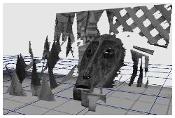
the image’s pixel grid. A visualization of the point cloud illustrated
in Figure 5 (right) which shows the view of the 3D Surface
generated from the disparity map and the camera calibration data.
The surface is also textured with the left camera image (here converted
to gray scale).
|
Adept Turnkey Pty Ltd are "The Machine Vision and Imaging
Specialists" and distributor of Machine Vision products in Australia
and New Zealand. To find out more about any machine vision product please
call us at Perth (08) 9242 5411 / Sydney (02) 9905 5551 / Melbourne
(03) 9384 1775 or contact us online.
|